Table of Contents
- Data Structures and Algorithams
An algorithm - Is a set of well-defined instructions to solve a particular problem. It takes a set of input and produces a desired output
- Input
- Output
- Definiteness - It must be clear
- Finiteness - It must stop
- Effectiveness - some purpose How to Analyse Alogithm
- Time - must be Time efficient
- Space - must be memory effficient
- N/W -
- Power -
- CPU Registers - Every statement/line is 1 unit of time Frequency Count Method
-
Means, the number of times the statement is executed in the program
-
To calculate the time, consider the degree
- sum(a,b) => f(n) = 2n +3 => O(n) - add(a,b,n) => f(n) = 2n2 + 2n + 1 => O(n2) - multiply(a,b,n) => f(n) = 3n3 + 3n2 + 2n + 1 => O(n3) -
To Calculate space complexity, consider all variables
- sum(a,b)      => s(n) = n+3        => O(n)
- add(a,b,n)  => s(n) = 3n2 + 3    => O(n2)
- multiply(a,b,n) => s(n) = 3n2 +4     => O(n2)
- for(i=0;i<n;i++)          => O(n)
- for(i=n;i>0;i--)          => O(n)
- for(i=0;i<n;i=i+2)    n/2 => O(n)
- for(i=0;i<n;i++)
    for(j=0;j<i;j++)        => O(n^2)
- for(i=1;i<n; i=i++)
  for(j=0;j<n;j++)          =>O(n^2)
- p=0
  for(i=0;p<=n;i++)         =>O(root N)

- for(i=1;i<n; i=i*2)       => O(log n base 2)
- for(i=1;i<n; i=i*3)       => O(log n base 3)
- for(i=n;i>1; i=i/2)       => O(log n base 2 )

- for(i=0;i*i<n;i++)        => O(root n)

- for(i=0;i<n;i++)          => O(n)
    stmt
  for(j=0;j<i;j++)
    stmt
- p=0
  for(i=0;i<n;i*2)          => O(log log n)
    stmt
  for(j=0;j<p;j*2)
 stmt

- for(i=0;i<n;i++)          =>O(nlogn)
    stmt
  for(j=0;j<i;j=n*2)
 stmt
- Time Complexity (how much runtime it will take)
- Space Complexity (how much memory it will take)
- Constant Time Complexity - O(1)
- Linear Time Complexity - O(n)
- Logarithmic Time Complexity - O(log n)
- Quadratic Time Complexity - O(n ** 2)
- Cubic Time Complexity - O(n ** 3)
- Exponential Complexity - O(2 power n)
- Mathematical way
- Programatic or Practical way
- Find the Fast increasing term
- Remove the cofficient in that term
1 < log n < √n < n < n log n < n2 < n3 ... 2n < 3n < Nn < O(1) < O(logN) < O(N) < O(NlogN) < O(N^2) < O(2^N)< O(N!)
- Logn n = 1
- logn 1 = 0
=> log(1) = 0
=> log(2) = 1
4 => 2 power 2                => log2(4)  =2
8 => 2 power 3                => log2(8)  =3
16 => 2 power 4               => log2(16) =4
1024 => 2 power 10            => log2(1024)=10
4,294,967,296 => 2 power 10   => log2(~4B)=32
- BigO Upper bound (f(n) <= BigO(n) )
- Omega Lower bound (f(n) >= Omega(g(n) )
- Theta Average bound (f(n) = Theta(n) )
- BigO or Omega is when we are not sure
- Theta gives best
- IF Theta can't find, go for BigO or Omega
Data Structures are way storing and organizing data in a computer for efficient access and modification
- Linear DS; in Python using List
- Similar data types - Stores data as contiguous memory locations
-
Linear DS, in Python using List
-
Stores as individual nodes and has pointers to next node
-
Singly-linked list:
- linked list in which each node points to the next node
- the last node points to null
-
Doubly-linked list:
- linked list in which each node has two pointers, p and n, such that p points to the previous node and n points to the next node;
- the last node's n pointer points to null
-
Circular-linked list:
- linked list in which each node points to the next node
- the last node points back to the first node
-
Time Complexity:
- Access: O(n)
- Search: O(n)
- Insert: O(1)
- Remove: O(1)
-
Diff
- For LL No need to allocate momory
- LL Insertion is easy
- LL Memory is higher (p & n)
- Insertion/Delete at begining = O(1)
- Insert/Delete at end = O(n)


-
Linear DS, Last In First Out operation;
- push - Insert at end
- pop - remove at end
- isEmpty - check stack empty
- isFull - check if stack is full
- peek - get the vale of top element (without remove)
-
In python using List/collections.deque/queue.LifoQueue
-
Time Complexity
- Push: Insert - O(1)
- Pop: Delete - O(1)
- Search - O(n)

-
Linear DS, First In First Out operation;
- push - Insert at end
- pop - remove at start
-
In python using List/collections.deque/queue.LifoQueue
-
Time Complexity
- Push: Insert - O(1)
- Pop: Delete - O(1)
- Search - O(n)
### Hashmap/Hashtable
-
Hashing
- assigning an object into a unique index called as key.
- Object is identified using a key-value pair
- Dictionary - collection of objects
-
Hash table storing elements as key-value pairs, identify using key
-
Hash table memory efficient
-
Lookp/Insertion/Deletion Complexity is using key always O(1)
-
Collision: if hash function generetes same function the conflict called Collision.
- Chaining - one key, store values as List in dictionary
- Open Addressing - Linear/Quadratic Probing and Double Hashing
- Linear Probing - collision is resolved by checking the next slot
- Quadratic Probing- similar to linear probing but the spacing between the slots is increased
- Double hashing - applying a hash function & another hash function
- Chaining - one key, store values as List in dictionary
-
Time Complexity:
- Lookp/Insertion/Deletion is using key always O(1)
-
- A Tree is Non Linear DS, hierarchical, undirected, connected, acyclic graph
- Root - top most node of a tree.
- Node - data and pointers to another node
- Edge - link between nodes
- leaf nodes(L1, L2, L3)
- Binary Tree
- parent node can have at most two children
- Left node has lesser numbers
- Right node has greater numbers
- Full Binary Tree - a tree in which every node has either 0 or 2 children
- Perfect Binary Tree - binary tree with exactly 2 child nodes at all level
- Complete Binary Tree - every level must be filled L & R, leaf node only lean towards left
- Pathological Binary Tree - tree having a single child either left or right
- Skewed Binary Tree - tree is either dominated by the left Pathological nodes or the right Pathological nodes
- Balanced Binary Tree - difference between the height of the left and the right is either 0 or 1
- Binary Search Tree
- Left subtree has lesser numbers,
- Right subtree has greater numbers
- BST every node has max 2 nodes
- Every Iteration we reduce space by half(1/2))
- if n=8 & 3 iterations, log 8 = 3 => O(log(n))
- Access, Insert, Search adn Delete = Θ(log(n))
- delete process
- if bst not empty => search for node => check node children
- delete node with children 0; simpley delete it
- delete node with children 1, replace with its child value then delete child
- delete node with children 2, replace largest value from left subnodes or smallest value from right subnodes
- Breadth first search
- level0, level1, level2(left to right), leve3(left to right)
- Depth first search
- In order traversal - left subtree, root, right subtree at each level)
- Pre order traversal - root, left subtree and right subtree at each level
- Post order traversal - left subtree, right subtree and root at each level
- smallest value - left most
- highest value - right most
- A Tree is Non Linear DS, hierarchical, undirected, connected, acyclic graph


- Non Linear DS, must Complete binary tree (every level must be filled L & R, leaf node only lean towards left) and should satisfy heap
- Binary heap
- Min heap - every level root node is lesser than childs
- Max Heap - every level root node is greater than childs
- Min heap - every level root node is lesser than childs
- Binomial heap
- Fibonaci heap
- Time Complexity:
- Access Max / Min: O(1)
- Insert: O(log(n))
- Remove Max / Min: O(log(n))


- A graph is Non Linear DS, a ordered pair of sets (V,E) vertices & edges
- Tree has root node but graph no root node
- Tree is only root to child. in graph any node to anynode possible
- Ex: google maps, GPS, facebook, LinkedIn, e-commerce web sites
- Graphs Direction Types
- Undirected Graph - edges are bidirectional (adjacency relation is symmetric)
- Directed Graph - edge are uni directional (adjacency relation is not symmetric)
- Complete Graph - all nodes should have path
- Graph Weight Types
- Weighted Graph: a graph some value/cost
- Unweighted Graph: a graph with no value/cost
- Graph Cycle Types
- Cyclic Graph - a graph has cycle
- Acylic Graph - a graph which does have any cycle. tree is acyclic graph
- Adjacent Nodes - if edge exists then called adjacent nodes
- Graph Path - sequence of vertices connected by edges
- Simple path - if all of its vertices are distinct
- closed path - first and last node is same
- Cycle - cycle is path, first & last node is same and all nodes to be distinct
- Graph Connectivity
- strongly connected - Directed & every node to node should have path
- weekly connected - connected but Undirected
- Degree of Node = number of edges its connected to it
- InDegree - Incoming number of edges
- OutDegree - outgoing number of edges
- Adjaceny Matrix - matrix (0 or 1) representation b/n the nodes
- Adjacency List - array of linked lists representation of a nodes
- In Python use dictionaries


- Traverse array using for loop, if not march then -1
- Time Complexity is O(n)


- Searching is based on n/2 iterations; - Iterative method - Recursive method - Ex: 10,14,19,26,27,31,33,35, 42, 44, 50 - Time Complexity is O(log n) ### Jump/block Search Algoritham - Like Linear Algorithms but - Typical time complexity O(√n). - Time Complexity is b/n (O(n)) and (O(log n))

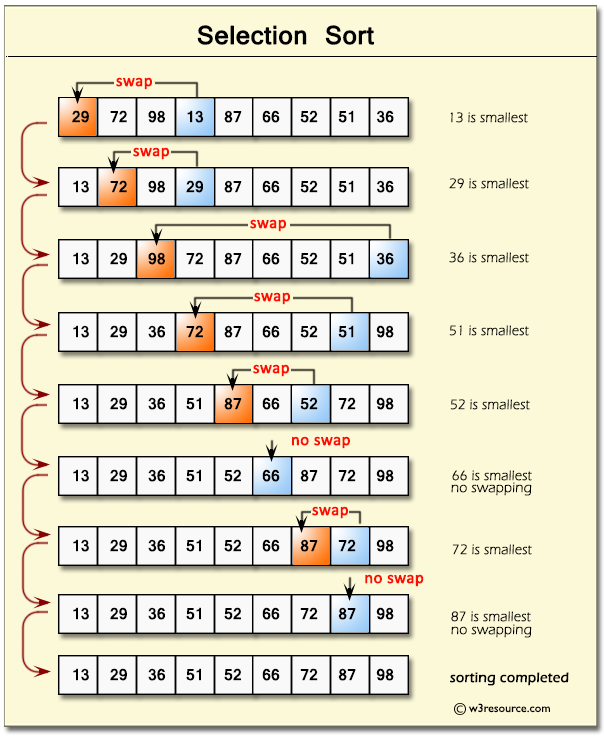
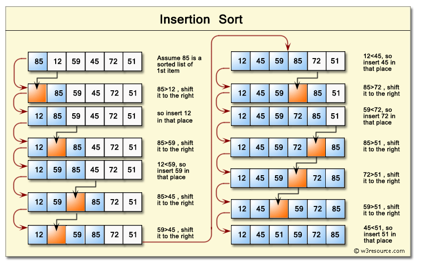
- Comparing adjacent items and swaps them untill intended order
- The loop untill all are sorted
-
- Time Complexity is O(n2)
- Time Complexity is O(n2)


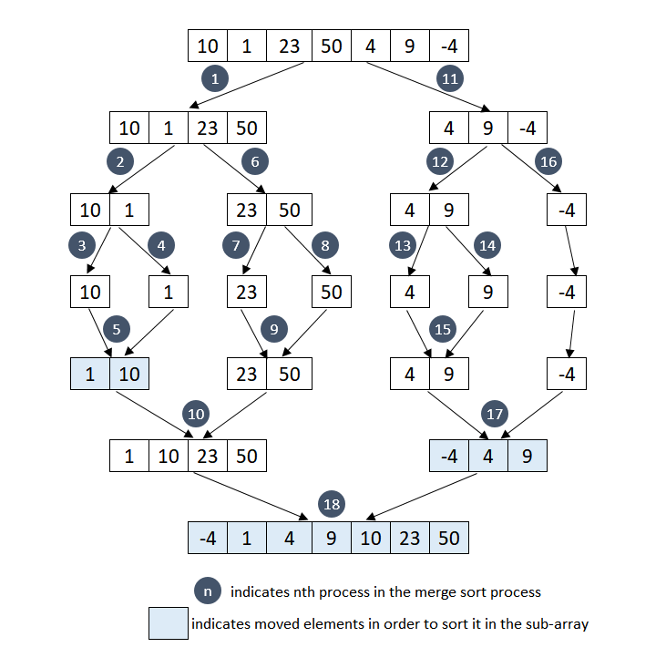

- Problem will be divded in to sub problems
- find solution for sub problem
- combine all solutions to one soluiton
- reucrisively solve
- binary search
- find min and max
- merge sort
- quick sort
- strassens matrix multiplication
-
Tries all the possibilities, chooses the desired/best solutions
-
Good Practice to come up with solution to all possible
-
least efficient but guaranteed a solution
-
Backtracking aproach
- find all the possible ways
-
State space tree
- define level by level
- top-down approach
- Greedy Choice Property
- choosing the best choice at each step
- most obvious and immediate benefit
- Optimal Substructure
- solution to its subproblems so that problem can be solved
-
- Greedy Choice Property


- technique to efficiently solve a class of problems that have overlapping subproblems
- problem can be divided into smaller subproblems
- if overlapping among subproblems, solution will be saved for future reference Ex: 0,1,1,2,3,5,8,13,21,34,55...(n-1 + n-2)
- https://www.bigocheatsheet.com/
- https://www.programiz.com/dsa/algorithm
- https://www.educative.io/blog/algorithms-an-interview-refresher#steps
- https://www.educative.io/blog/python-dynamic-programming-tutorial#dp
- https://leetcode.com/discuss/general-discussion/460599/blind-75-leetcode-questions
- https://github.com/kdn251/interviews#youtube
- https://github.com/TheAlgorithms/Python/blob/master/DIRECTORY.md
- https://github.com/prabhupant/python-ds
- https://www.geeksforgeeks.org/data-structures/?ref=shm
- https://github.com/tayllan/awesome-algorithms#websites
- https://github.com/prabhupant/python-ds
- https://github.com/TheAlgorithms/Python/blob/master/DIRECTORY.md
- https://github.com/vinta/fuck-coding-interviews
- https://github.com/teivah/algodeck/
- https://docs.google.com/spreadsheets/d/1pEzcVLdj7T4fv5mrNhsOvffBnsUH07GZk7c2jD-adE0/edit#gid=0